covariates_plot() produces a plot of the covariates' effects (\(\hat\beta\))
with confidence intervals, or of the Hazard Ratios (\(\exp(\hat\beta)\)) with confidence intervals.
Usage
covariates_plot(
  fitted_model,
  confidence_lev = 0.95,
  plot_options = list(),
  ...
)
Arguments
- fitted_model
A list returned by the function
fit2ts(),fitpgam()orfit1ts().- confidence_lev
The level of confidence for the CIs. Default is 0.95 (\(\alpha = 0.05\)).
- plot_options
A list of options for the plot:
HRA Boolean. IfTRUEthe HRs with their CIs will be plotted. Default isFALSE(plot thebetawith their CIs).symmetric_ciA Boolean. Default isTRUE. If a plot of the HRs is required (HR == TRUE), then plot symmetrical Confidence Intervals, based on the SEs for the HRs calculated by delta method. IfFALSE, then CIs are obtained by exponentiating the CIs for the betas.mainThe title of the plot.ylabThe label for the y-axis.ylimA vector with two elements defining the limits for the y-axis.col_betaThe color for the plot of the covariates' effects.pchThe symbol for plotting the point estimates.cex_mainThe magnification factor for the main of the plot.
- ...
further arguments passed to plot()
Value
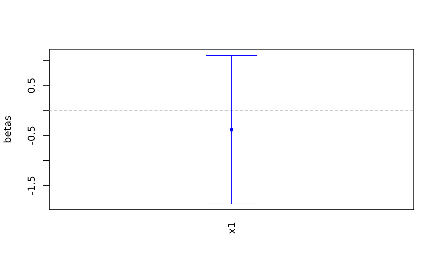
A plot of the covariates' effects. The different covariates are plotted on the x-axis, and on the y-axis the effects on the coefficient- or on the HR-scale are plotted. The main estimate is represented by a point and the CIs are added as vertical bars.
Examples
# Create some fake data - the bare minimum
id <- 1:20
u <- c(
5.43, 3.25, 8.15, 5.53, 7.28, 6.61, 5.91, 4.94, 4.25, 3.86, 4.05, 6.86,
4.94, 4.46, 2.14, 7.56, 5.55, 7.60, 6.46, 4.96
)
s <- c(
0.44, 4.89, 0.92, 1.81, 2.02, 1.55, 3.16, 6.36, 0.66, 2.02, 1.22, 3.96,
7.07, 2.91, 3.38, 2.36, 1.74, 0.06, 5.76, 3.00
)
ev <- c(1, 0, 0, 1, 0, 1, 0, 1, 1, 0, 1, 0, 0, 1, 0, 0, 0, 0, 0, 1)
x1 <- c(0, 0, 0, 1, 0, 1, 1, 1, 1, 0, 0, 0, 1, 0, 1, 1, 0, 0, 1, 0)
fakedata <- as.data.frame(cbind(id, u, s, ev, x1))
covs <- subset(fakedata, select = c("x1"))
fakedata2ts <- prepare_data(
u = fakedata$u,
s_out = fakedata$s,
ev = fakedata$ev,
ds = .5,
individual = TRUE,
covs = covs
)
#> `s_in = NULL`. I will use `s_in = 0` for all observations.
#> `s_in = NULL`. I will use `s_in = 0` for all observations.
# Fit a fake model - not optimal smoothing
fakemod <- fit2ts(fakedata2ts,
optim_method = "grid_search",
lrho = list(
seq(1, 1.5, .5),
seq(1, 1.5, .5)
)
)
# Covariates plot with default options
covariates_plot(fakemod)
 #> [1] 1
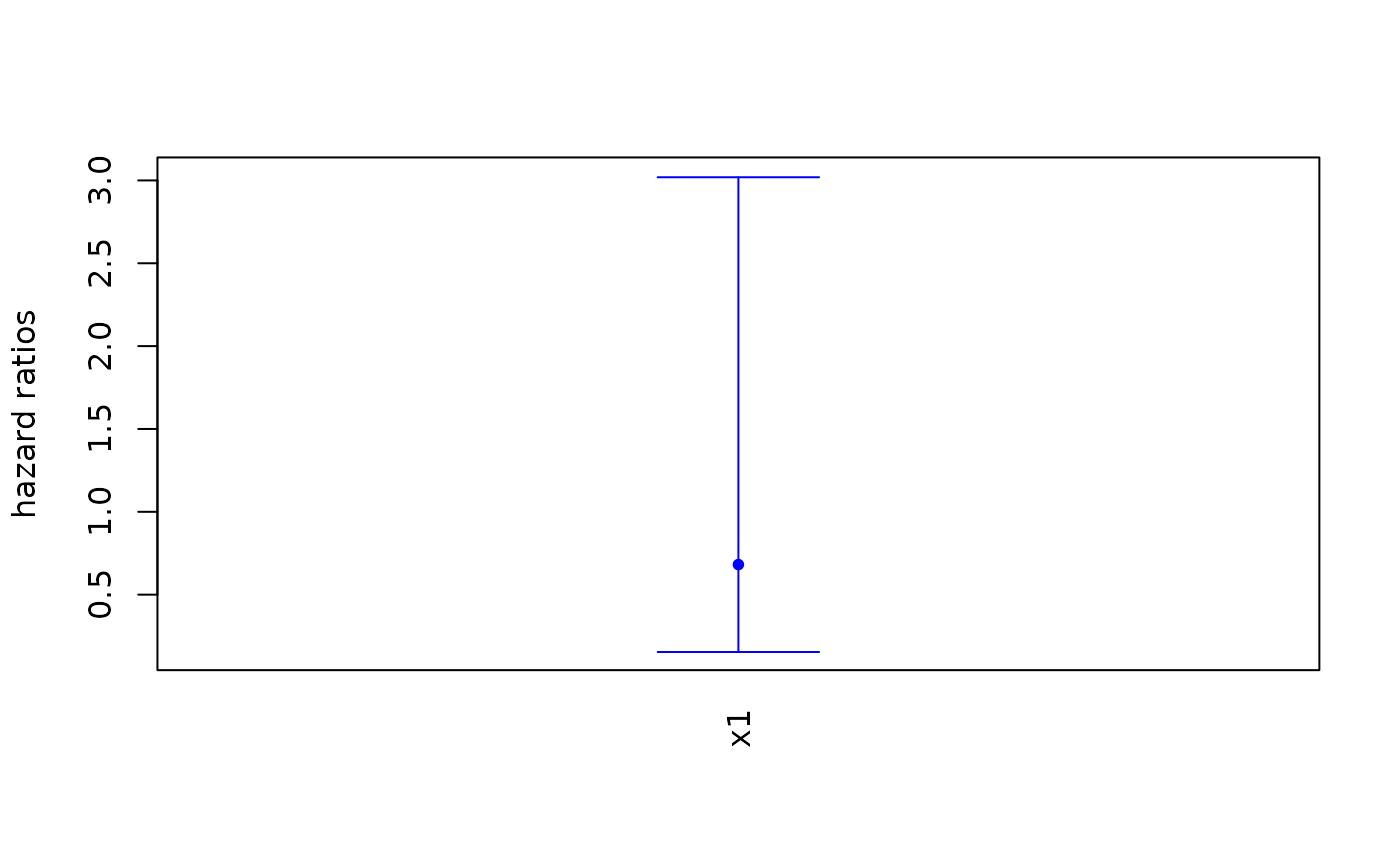
# Plot the hazard ratios instead
covariates_plot(fakemod,
plot_options = list(
HR = TRUE
)
)
#> [1] 1
# Plot the hazard ratios instead
covariates_plot(fakemod,
plot_options = list(
HR = TRUE
)
)
 #> [1] 1
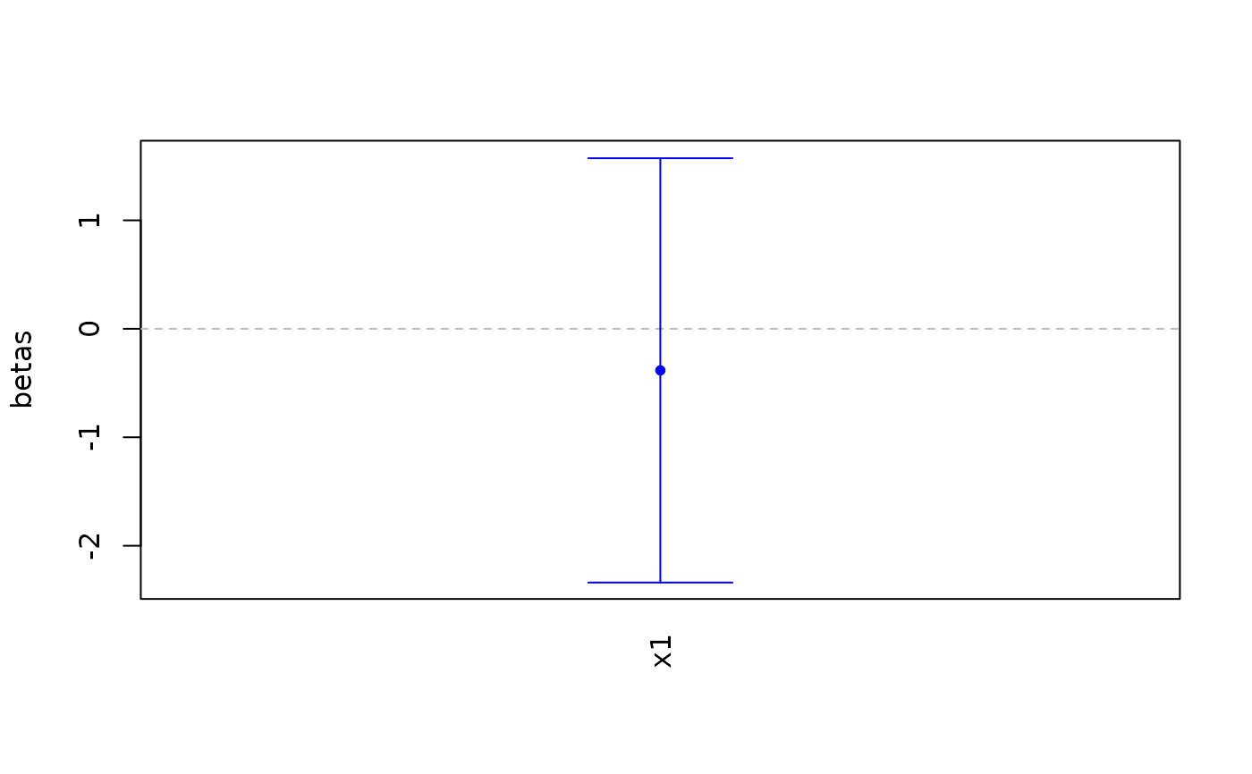
# Change confidence level
covariates_plot(fakemod,
confidence_lev = .99
)
#> [1] 1
# Change confidence level
covariates_plot(fakemod,
confidence_lev = .99
)
 #> [1] 1