Smooth hazards with one time scale

library(TwoTimeScales)

We assume that the reader of this vignette has some familiarity with the $P$-splines model for the hazard, and with the basic functions of the package introduced in the vignette Introduction to TwoTimeScales.

This vignette demonstrates in detail how to use the package TwoTimeScales to estimate a smooth hazard model with one time scale, and how to plot the estimates. We use the dataset reccolon2ts included in the package, and we analyse mortality after recurrence of the colon cancer, over time since recurrence. For an overview of the data use: help(reccolon2ts).

Data preparation

The first step of the analysis, is data preparation. Data are in wide format, with one row for each patient. To estimate a $P$-spline model for the hazard we need to bin the individual data, that is exposure times and event counts, into many small bins of equal size, that cover the whole range of values for the time scale. Data preparation involves the construction of the bins and the actual binning of the data. Both steps are implemented and performed by the function prepare_data(), which requires as inputs the individual data vectors and the desired specification for the bins. The function returns an object of type data2ts.The print method can be used to analyse the structure of the resulting object.

First, we show how the function works with minimal input (that is, by using the default values for any optional parameter):

dt1ts <- prepare_data(data = reccolon2ts,
                      s_out = "timesr",
                      events = "status",
                      ds = 30)

> str(dt1ts)
List of 2
 $ bins   :List of 3
  ..$ bins_s: num [1:92] 0 30 60 90 120 150 180 210 240 270 ...
  ..$ mids  : num [1:91] 15 45 75 105 135 165 195 225 255 285 ...
  ..$ ns    : int 91
 $ bindata:List of 2
  ..$ r: num [1:91] 13674 13070 12474 12002 11534 ...
  ..$ y: num [1:91] 14 24 16 11 24 22 20 10 24 26 ...
 - attr(*, "class")= chr "data2ts"

> print(dt1ts)
An object of class 'data2ts'

Data:
List of 2
 $ bins   :List of 3
 $ bindata:List of 2
 - attr(*, "class")= chr "data2ts"
NULL

Range covered by the bins: 
$bins_s
[1]    0 2730


Number of bins: 
$ns
[1] 91


Overview of the binned data:
Total exposure time: 246018
Total number of events: 409

The function requires as minimal inputs only a vector of exit times (s_out), a vector of event’s indicators (events) and the desired bins’ size (ds). The object dt1ts is a list with two elements. The first element is a list of bins (bins_s) with their midpoints (mids) and the total number of bins (ns). The second element of the list is another list with the data binned, a vector of exposure times called r and a vector of counts of events y.

We notice that the calling generated the message s_in = NULL. I will use s_in = 0 for all observations.; this message is informing the user that a vector of entry times was not provided. It is assumed that the entry times are not left truncated (everyone is observed from the beginning of the process), and considering s_in = 0 is therefore correct. As explained in the introductory vignette, we included some artificial left truncated times for the entry into the risk set. In fact, when we use the variable that includes left truncation, the message disappears:

dt1ts_lt <- prepare_data(data = reccolon2ts,
                         s_in = "entrys",
                         s_out = "timesr",
                         events = "status",
                         ds = 30)

Without specifying additional inputs, the constructions of the bins is done by covering the minimum range of values for the time scale, with bins of desired size ds. We can change the width of the bins by changing the argument ds. For example, the following code builds one bin each 90 days, approximately 3 months. As consequence, the number of bins is about 3 times less than in the previous case.

dt1ts_lt2 <- prepare_data(data = reccolon2ts,
                          s_in = "entrys",
                          s_out = "timesr",
                          events = "status",
                          ds = 90)

> dt1ts_lt2$bins$ns

[1] 31

It is also possible to specify minimum and maximum values for the bins. This option can be helpful when, for example, the event times are left-truncated but it is still desirable to have bins starting at 0.

> range(reccolon2ts$timesr)

[1]    3 2725

dt1ts_2 <- prepare_data(data = reccolon2ts,
                        s_in = "entrys",
                        s_out = "timesr",
                        events = "status",
                        ds = 30, min_s = 0, max_s = 3000)

> str(dt1ts_2)

List of 2
 $ bins   :List of 3
  ..$ bins_s: num [1:101] 0 30 60 90 120 150 180 210 240 270 ...
  ..$ mids  : num [1:100] 15 45 75 105 135 165 195 225 255 285 ...
  ..$ ns    : int 100
 $ bindata:List of 2
  ..$ r: num [1:100] 12613 12322 11793 11399 10969 ...
  ..$ y: num [1:100] 14 24 16 11 24 22 20 10 24 26 ...
 - attr(*, "class")= chr "data2ts"

Now 100 bins have been created, spanning the range from 0 days to 3000 days of follow-up.

When the aim of the analysis is to estimate a proportional hazard model, a different structure of the data is required (Carollo et al. (2024)). In particular, when only one time scale is considered, we need to create a matrix of exposure times R with dimension n (number of individuals in the data) by ns (number of bins). Similarly for the matrix of event counts. The function prepare_data() returns data with this structure by specifying the optional input individual = TRUE. It is possible, and recommended, to provide the names of the covariates that one wishes to use in the PH model in the extra argument covs. The function will take care of the preparation of the regression matrix Z. However, if desired, this can also be prepared externally (in which case a warning will be returned).

dt1ts_cov <- prepare_data(data = reccolon2ts,
                          s_in = "entrys",
                          s_out = "timesr",
                          events = "status",
                          ds = 30,
                          individual = TRUE, 
                          covs = c("rx", "node4", "sex"))

> print(dt1ts_cov)

An object of class 'data2ts'

Data:
List of 2
 $ bins   :List of 3
 $ bindata:List of 3
 - attr(*, "class")= chr "data2ts"
NULL

Range covered by the bins: 
$bins_s
[1]    0 2730


Number of bins: 
$ns
[1] 91


Overview of the binned data:
Total exposure time: 236006
Total number of events: 409
Covariates:
[1] "rx_Lev"     "rx_Lev+5FU" "node4"      "sex_male"  

From print(dt1ts_cov), we see that 4 covariates are included in the Z regression matrix. The variable rx includes 3 categories, and it is therefore represented in the regression matrix by two dummy variables (rx_Lev and rx_Lev+5FU).

Estimation

First, we show how to estimate a model without covariates. The proportional hazard model is introduced in a second step. The function that estimates the model is fit1ts(), that is a wrap around several other functions, performing the estimation. The estimation is done in two steps: First, given a set of values for the smoothing parameter, or one single starting value, a search for the model with minimum AIC (or BIC) is performed. Once the model with minimum AIC (or BIC) is identified, the optimal smoothing parameter is selected and the optimal model is finally estimated.

For details of each argument of fit1ts() we refer to the manual or the function documentation, which can be accessed by help("fit1ts"). Here, we show how to modify the different arguments to estimate the one time scale model in different ways.

The only required argument is data1ts, which is an object returned by the function prepare_data(), as we have seen in the previous section. When this argument, and no other argument is passed to fit1ts(), estimation is performed with all the default options. In most scenarios, the user will want to use prepare_data() to perform data preparation and then directly pass the output of prepare_data() to fit1ts(). However, if the available data are already aggregated into vectors of event’s counts and exposure times, the user can pass these as arguments to fit1ts(), to y and r respectively. In this case is necessary to provide values for bins too, and it is important that all three arguments are provided and that the length of y, r and bins$mids are the same.

First, we only pass as argument the object dt1ts, which was created before. Then, we show, only as illustration, how the same estimates of the $\alpha$ are obtained when we pass the arguments y, r and bins, taken from the same object.

# Model 1 - Default parameters (numerical optimization of aic, default param for
#                               B-splines)
m1 <- fit1ts(data1ts = dt1ts)
# Model 2 - Single data inputs
m2 <- fit1ts(y = dt1ts$bindata$y, r = dt1ts$bindata$r, bins = dt1ts$bins)

> table(m1$optimal_model$alpha == m2$optimal_model$alpha)

TRUE 
  13 

> str(m1)

List of 3
 $ optimal_model :List of 9
  ..$ alpha   : num [1:13, 1] -6.96 -6.57 -6.22 -6.14 -6.28 ...
  ..$ SE_alpha: num [1:13] 0.3466 0.1197 0.0893 0.0983 0.1221 ...
  ..$ eta     : num [1:91, 1] -6.55 -6.51 -6.48 -6.44 -6.4 ...
  ..$ H       : num [1:13, 1:13] 0.16707 0.0782 0.00508 -0.01083 -0.00517 ...
  ..$ deviance: num 79.8
  ..$ ed      : num 4.04
  ..$ aic     : num 87.9
  ..$ bic     : num 98.1
  ..$ Bbases  :List of 1
  .. ..$ Bs: num [1:91, 1:13] 0.1407 0.0971 0.0636 0.0388 0.0215 ...
  .. .. ..- attr(*, "x")= num [1:91] 15 45 75 105 135 165 195 225 255 285 ...
  .. .. ..- attr(*, "xl")= num 0
  .. .. ..- attr(*, "xr")= num 2730
  .. .. ..- attr(*, "nseg")= num 10
  .. .. ..- attr(*, "bdeg")= num 3
  .. .. ..- attr(*, "type")= chr "bbase"
 $ optimal_logrho: num 1.13
 $ P_optim       : num [1:13, 1:13] 13.4 -26.8 13.4 0 0 ...
 - attr(*, "class")= chr "haz1ts"

The object returned by fit1ts() is of class 'haz1ts'. The first element is a list with the results of the optimal model. The second element is the optimal smoothing parameter (on the $\log_{10}$-scale) and the last element is the penalty matrix P_optim, incorporating the optimal value of $\varrho$.

In the following examples we show how to modify the arguments of the function, to obtain slightly different model specifications. The results are not shown here, but we encourage the reader to run these examples on their console.

# Model 3 - Change specifications of the B-splines (degree, number of segments 
#                                                   and range)
m3 <- fit1ts(data1ts = dt1ts,
             Bbases_spec = list(bdeg = 2,          # quadratic B-splines
                                nseg_s = 20,       # 20 segments
                                min_s = 0,         
                                max_s = 2730))

# Model 4 - As m3, but change penalty order
m4 <- fit1ts(data1ts = dt1ts,
             Bbases_spec = list(bdeg = 2,
                                nseg_s = 20,
                                min_s = 0,
                                max_s = 2730),
             pord = 3)                             # third-degree penalty

# Model 5 - As m3, but change optimization method to grid_search
m5 <- fit1ts(data1ts = dt1ts,
             Bbases_spec = list(bdeg = 2,
                                nseg_s = 20,
                                min_s = 0,
                                max_s = 2730),
             optim_method = "grid_search")         # search for optimal smoothing                                                                           over grid of values

# Model 6 - As m5, but optimization criterion is "bic" and include grid of 
#           values for log_10(rho)
m6 <- fit1ts(data1ts = dt1ts,
             Bbases_spec = list(bdeg = 2,
                                nseg_s = 20,
                                min_s = 0,
                                max_s = 2730),
             optim_method = "grid_search",
             optim_criterion = "bic",              # use BIC rather than AIC
             lrho = seq(-2, 3, by=.2))             # provide grid for log_10(rho)

Finally, we demonstrate how to plot the AIC and BIC curves, mark the optimal values of the smoothing parameter, and extract the AIC and BIC vectors after a grid search of the optimal smoothing parameter.

par(mfrow = c(1,2))
m6 <- fit1ts(data1ts = dt1ts,
             Bbases_spec = list(bdeg = 2,
                                nseg_s = 20,
                                min_s = 0,
                                max_s = 2730),
             optim_method = "grid_search",
             optim_criterion = "bic",
             lrho = seq(-1, 3, by=.2),
             par_gridsearch = list(
               plot_aic = T,
               plot_bic = T,
               mark_optimal = T
             ))
par(mfrow = c(1,1))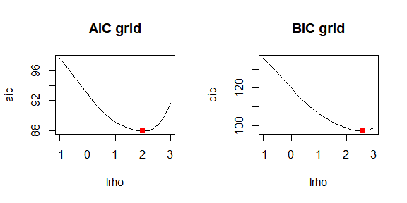

m6.aic <- m6$AIC
m6.bic <- m6$BIC

> m6.aic[1:6]; m6.bic[1:6]

[1] 97.67005 96.78100 95.81061 94.79922 93.79740 92.84326
[1] 135.6309 132.7852 129.7015 126.4681 123.1973 119.9904

We notice how, for the same data and over the same grid of $\log_{10}(\varrho)$ values, the BIC criterion selects a larger smoothing parameter than the AIC. This behavior is well known, as the BIC penalizes differences in neighboring coefficients more strongly than AIC, leading to smoother results.

Finally, we estimate a PH model including the covariates rx, node4 and sex, and see how to extract the estimates of the regression parameters $\beta$s.

m7 <- fit1ts(data1ts = dt1ts_cov,
             Bbases_spec = list(nseg_s = 15,
                                min_s = 0,
                                max_s = 2730))
betas <- m7$optimal_model$beta

> betas
    rx_Lev rx_Lev+5FU      node4   sex_male 
0.07875399 0.27900614 0.50543144 0.21322565 

In the next section, we will show how to get estimates of the (log-)hazard curve with one time scale, using the same $B$-splines basis as for the estimation, or evaluating this old basis in a denser grid. We will also see how to obtain estimates of the hazard ratios, and how all these steps can be performed jointly and plotted using the function plot().

Presenting the results of the smooth one time scale hazard model

We will explore several options for the presentation of the results of the one time scale model, using the last model we estimated in the previous section, which included four covariates. The object returned by fit1ts() provides the estimates of both the parameters of the $B$-splines, that is a vector of $\hat{\alpha}$ values, and the estimates of the covariates’ effects, a vector of $\hat{\beta}$ values. The hazard is obtained from the $\hat{\alpha}$ by multiplying each coefficient to the corresponding $B$-spline, summing up the contributions of each scaled $B$-spline in a specific point and finally exponentiating the result: $$\hat\lambda = \exp\left\{\sum^{n_s}_{k=1} b_{kl}\alpha_l\right\}.$$

The function get_hazard_1d() returns a vector of estimates for the (log-)hazard, and the associated standard errors, given as input the object returned by fit1ts() and, optionally, a list of specifications for evaluating the $B$-splines basis on a new grid. When applied to a PH model, it returns the baseline hazard.

We show how to provide specifications for the $B$-splines and how to use the function get_hazard_1d(). We will evaluate the $B$-splines basis on a finer grid, where the distance between the bins is of 10 days.

basehaz <- get_hazard_1d(fitted_model = m7,
                         plot_grid = c("smin" = 0, "smax" = 2730, "ds" = 10))

> str(basehaz)

List of 7
 $ new_plot_grid :List of 4
  ..$ ints: num [1:274] 0 10 20 30 40 50 60 70 80 90 ...
  ..$ smin: Named num 0
  .. ..- attr(*, "names")= chr "smin"
  ..$ smax: Named num 2730
  .. ..- attr(*, "names")= chr "smax"
  ..$ ds  : Named num 10
  .. ..- attr(*, "names")= chr "ds"
 $ hazard        : num [1:274, 1] 0.00095 0.000964 0.000978 0.000992 0.001007 ...
 $ loghazard     : num [1:274, 1] -6.96 -6.94 -6.93 -6.92 -6.9 ...
 $ log10hazard   : num [1:274, 1] -3.02 -3.02 -3.01 -3 -3 ...
 $ SE_hazard     : num [1:274, 1] 0.000169 0.000168 0.000166 0.000165 0.000164 ...
 $ SE_loghazard  : num [1:274, 1] 0.178 0.174 0.17 0.166 0.163 ...
 $ SE_log10hazard: num [1:274, 1] 0.0775 0.0756 0.0738 0.0721 0.0706 ...

> range(basehaz$hazard)

[1] 0.000191134 0.001517088

The calls returns a list with several elements: The new grid for plotting new_plot_grid, a vector for the hazard values hazard, a vector for the log-hazard values loghazard , a vector with the $log_{10}$-hazard values log10hazard and three vectors with the associated standard errors, respectively SE_hazard, SE_loghazard ans SE_log10hazard. The hazard ratios and their standard errors are obtained by calling the function get_hr:

hr <- get_hr(fitted_model = m7)

> hr$HR

    rx_Lev rx_Lev+5FU      node4   sex_male 
  1.081938   1.321815   1.657701   1.237664 

It is possible to call these two functions independently and to use the resulting objects to create a plot of the results. However, this is exactly what is done by the method plot(), implemented for objects of class 'haz1ts'.

plot(m7)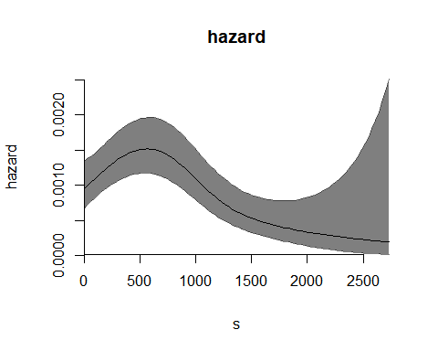

This simple call produces, for a PH model, the plot of the baseline hazard curve. Now we interpolate the $B$-spline basis on a denser plotting grid, and change other parameters to obtain a nicer plot.

plot(m7,
     plot_grid = c("smin" = 0, "smax" = 2730, "ds" = 10),
     plot_options= list(
       col = "purple",
       main = "Baseline hazard",
       ylab = "hazard",
       xlab = "time since recurrence",
       cex_main = 1))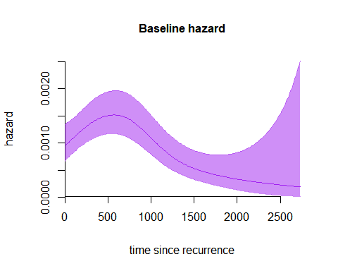

The hazard can also be plotted on the log-scale, by setting the argument plot_options$loghazard = TRUE:

plot(m7,
     plot_grid = c("smin" = 0, "smax" = 2730, "ds" = 10),
     plot_options= list(
       loghazard = TRUE,
       col = "purple",
       main = "Baseline hazard",
       ylab = "log-hazard",
       xlab = "time since recurrence",
       cex_main = 1))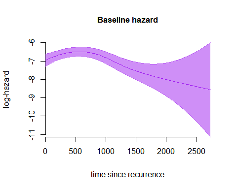

We can also plot the covariate effects by calling:

plot(m7,
     which_plot = "covariates")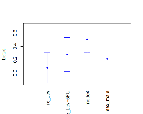

This call plots the point estimates for the $\beta$ parameters with their 95% confidence intervals. Alternatively, we can decide to plot the estimated hazard ratios, with their confidence intervals. There are two options regarding the confidence intervals for the HRs: First, we can use the delta method to find confidence intervals that are symmetric around the HRs estimates. Second, we can exponentiate the confidence intervals for the $\beta$ parameters, and therefore obtain non-symmetric (but always positive) confidence intervals for the HRs. We show both options here:

par(mfrow = c(1,2),
    font.main = 1)
# Option 1: symmetric CIs with delta method
plot(m7,
     which_plot = "covariates",
     plot_options = list(
       HR = T,
       symmetric_CI = T,
       ylim = c(0.8, 2.1),
       main = "HR with symmetric CIs",
       cex_main = 1
     ))
abline(h=1, lty=2, col="grey")
# Option 2: non-symmetric CIs 
plot(m7,
     which_plot = "covariates",
     plot_options = list(
       HR = T,
       symmetric_CI = F,
       ylim = c(0.8, 2.1),
       main = "HR with non-symmetric CIs",
       cex_main = 1
     ))
abline(h=1, lty=2, col="grey")
par(mfrow = c(1,1))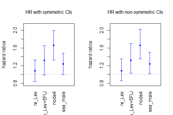

Finally, it is possible to change the level of confidence for the CIs. In the following we show three different levels for the same $\beta$.

par(mfrow = c(1,3),
    font.main = 1)
plot(m7,
     which_plot = "covariates",
     plot_options = list(
       ylim = c(-0.22, 0.8),
       main = "95% CIs",
       cex_main = 1
     ))
abline(h=0, lty=2, col="grey")
plot(m7,
     which_plot = "covariates",
     plot_options = list(
       ylim = c(-0.22, 0.8),
       confidence = .90,
       main = "90% CIs",
       cex_main = 1
     ))
abline(h=0, lty=2, col="grey")
plot(m7,
     which_plot = "covariates",
     plot_options = list(
       ylim = c(-0.22, 0.8),
       confidence = .99,
       main = "99% CIs",
       cex_main = 1
     ))
abline(h=0, lty=2, col="grey")
par(mfrow = c(1,1))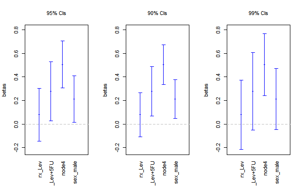

# References

Carollo, Angela, Paul H. C. Eilers, Hein Putter, and Jutta Gampe. 2024. “Smooth Hazards with Multiple Time Scales.” Statistics in Medicine. https://doi.org/10.1002/sim.10297.